The Art Gallery Problem: Mathematical analysis of area coverage

Often times while doing a security analysis of a physical area, I am interested in the efficient placement of assets to monitor and secure an area. In mathematics the placement of security resources within an area is often modeled as a geometric area coverage problem. We can restate our problem as "What is the minimum number of resources required to cover the inside of a given polygon".  Today I will discuss a software for analyzing and planning physical security layouts based off of the insights revealed by studying this problem.

Problem Description

A formal  problem definition is known as the Art Gallery Problem (AGP). From the Wikipedia entry you can learn AGP (a.k.a. the museum problem) is a well-studied visibility problem in computational geometry. It originates from a real-world problem, which it's name is derived from, of guarding an art gallery with the minimum number of guards which would allow the guards together to observe the whole gallery. One well-known theorem on the problem was posed by Computer Scientist and Professor, Václav Chvátal. Chvátal AGP theorem gives an upper bound that states "At most n/3 guards is always sufficient, and sometimes required, to cover a polygon with n vertices". His work was later simplified by Steve Fisk who reduced the problem to a 3-coloring problem. I will be using the geometric version of the problem, in which the layout of the art gallery is represented by a set of polygons. Each guard and device is represented by a point within (or on the edge of) the polygon.

"A set ${\displaystyle S}$S of S points is said to guard a polygon if, for every point ${\displaystyle p}$p in the polygon, there is some ${\displaystyle q\in S}$ q subset S such that the line segment between ${\displaystyle p}$p and q ${\displaystyle q}$ does not leave the polygon." - Art Gallery Problem Wiki

Chvátal's upper bound remains true, even if the restriction of "guards at corners" is loosened to "guards anywhere within the interior of the polygon".

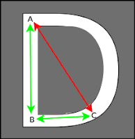
To simplify things at first, the problem assumes the resource can view all of the area not obscured by the vertices of a wall. In reality, a scaling factor should be applied. For example, in the above diagram, if the straight section between the green zone and the blue zone is 10 feet maybe the overlap is reasonable. However if it is 100 feet or more, maybe the overlap is not as reasonable. If the resource we are discussing is a human security guard in a potentially crowded gallery, could they really see into a corner down a hallway more than 100 ft away?
  When the AGP is defined as described above, finding the optimal solution will be NP-complete, this because a suggested solution can be verified in polynomial time, while finding the optimal solution can only be done by testing all possible candidates. Chvátal's theorem proved that n/3 is always enough (and at times required) to guard the entire polygon, as mentioned above. There is no guarantee that this number of guards is optimal when using this approach.

Definitions

A number of definitions are needed to set up the parameters of the problem. These are taken directly from the paper:

Simple polygon

A simple polygon is a closed plane figure whose boundary, Pbd, is composed of straight line edges, and where no two non-consecutive edges intersect. The points are referred to as the vertices of P.

Simple polygon with holes

P may contain holes. These are then represented as simple polygons without holes enclosed by Pbd. The term simple polygon is reserved for simple polygons without holes. If the polygon may contain holes, the term simple polygon with holes is used.

Orthogonal polygon

An orthogonal polygon is a polygon that has a 90° angle between the two edges that intersect at each vertex. The term orthogonal polygon refers to an orthogonal polygon that is also simple. Orthogonal polygons with holes is used to refer to simple polygons with holes where both the main polygon and its holes are orthogonal.

Visibility in a polygon

Simple Polygon with hole visibility example

Two points p and q of polygon P are said to be visible from each other if the line segment from p to q lies completely in P. If P has holes, the line segment cannot intersect with any part of the hole.

Algorithm Notes

In a 2008 thesis paper "The Camera Placement Problem– An art gallery problem variation", Mikael Pålsson and Joachim Ståhl examine the 3-color algorithm and propose a set of alternate 'rectangular' algorithms specifically designed with camera placement in mind. They deal with the shortcomings of camera range, angle and obstructions. I will be using a blend of the Chvátal and the Pålsson/Ståhl approaches to the problem. Pålsson/Ståhl were able to address several practical pitfalls to Chvátal's theorem. According to their research goals, an algorithm that solves the camera placement problem should be able to handle the following:

• Limited field of view of cameras.
• Limited effective range of cameras.
• Obstacles limiting the line of sight, also called polygon holes.
• A coverage threshold.

These goals make the placement selection more realistic. There are still several other constraints that can/should be filled. These include the ability to weight areas to determine the required coverage. For example, a bank may weight the monitoring of private offices lower than that of the lobby. Another type of constraint may be that each camera has to be visible to at least one other camera. This is helpful to prevent vandalism or blind spots below the camera. While I do not plan to implement all of these constraints, it is helpful to frame the problem in this way. A primary drawback to the Pålsson/Ståhl approach is the simplification to orthogonal polygons. It is true that many spaces can be modeled (or closely approximated) using orthogonal polygons, but the limitation makes it impractical for general use in planning physical security layouts.

Floor Plans are a mix of orthogonal and simple polygons

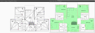
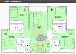
To blend the two approaches, I create a program which allows a user to draw 1 or more polygons (with holes) representing the area(s) to be guarded.

Polygons drawn over a Floor Plan

Each polygon is then tessellated with the Delaunay triangulation algorithm available in the Scipy.Spacial library. The vertices defining each polygon and the resulting triangulation are then turned into a NetworkX Graph. The graph nodes are then colored using the networkx.algorithms.coloring.greedy_coloring algorithm.

Delaunay Triangulation of each room

Potential perimeter locations are selected by taking all nodes of a particular color. Often times the color with the fewest nodes is chosen for each room. After applying scaling, I can define devices using common parameter such as Field of View, Effective Range, and Rotation to generate a polygon approximating the maximum visibility area for each device.

Two devices added with FoV polygons

Interior Guards and Areas of Responsibility

So far I have only considered points at the vertices of each polygon. By adding Interior Guards, a user can section a space into Areas of Responsibility. Generally speaking a guard is responsible for the part of the space that is closer to him than any other guard. A Voronoi Diagram shows exactly this information by finding the dividing vertices between three or more points in a 2D plane. These vertices are then connected and extended to create cells which contain exactly 1 guard point.

Voronoi Diagram to approximate AoR coverage

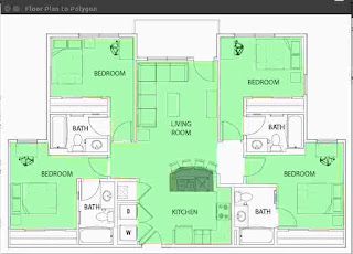
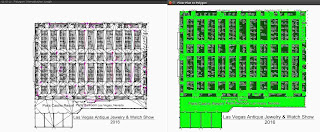
A more practical application can be seen in the example below. I found a Floor Plan drawing for the ballroom section of the Paris Hotel in Las Vegas.  This floor plan shows the setup of temporary booths. These obstructions and various openings make for a much more complex shape to consider. The first practical choice is how detailed to trace the polygon. I prefer to put points at bends or major security concerns (like doors and windows). The number and position on the vertices in obstructions also impacts the output.

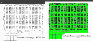Converting the Floor Plan into a Polygon with holes

Once I traced the base polygon and added obstructions for each of the booth clusters, I generated the Delaunay triangulation for the shape. I use the aforementioned coloring algorithm to select a starting color for each node.

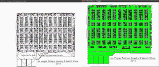Delaunay Triangulation of the resulting shape

By taking the color with the fewest vertices we come up with the Magenta layout below. Selecting the least-occurring color for each polygon's triangulation equates to finding nodes with higher connectivity. This is because the coloring algorithm will only add a new color if a node is already connected to nodes of each previous color.

Node and edges for least-used color

Of course, an area so large couldn't be covered by exterior sensors alone. I added interior guards in a reasonable pattern and generated the Areas of Responsibility chart below. By looking at the AoR distribution below, one may conclude that 1-3 more guards in the bottom portion of the map would help break the large sections up better. Mathematically this can be achieved by taking the area of each Voronoi cell, where it overlaps the main polygon. I start by placing a new guard in the center of the top n cells (by area). I then check to make sure these points are contained within a room polygon. If any guard is not within a room polygon, I adjust the position toward the closest base polygon and check again. This eventually yields all points within each cell that is within a room polygon. Finally I use the new layout to calculate the adjusted Areas of Responsibility.

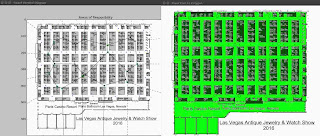Areas of Responsibility from interior guard placement

Other Interesting Bits

Aside from the core problem of writing a software to handle translating 2D spaces into a data structure appropriate for analysis there were several sub-problems that posed interesting learning opportunities.

Pythagorean Theorem

This one sent me back to my reference material. One might assume since I use triangulation fairly regularly that I have memorized the underlying math. How wrong they would be. With access to good software libraries it is easy to forget the theorem that underpins what we are working on.

Programmatically, you can just create the shape from it's point tuples and then use the geometry library shapely to find the area. There is another area where triangulation reared it's head. When defining devices, I mentioned a Field of View attribute and a Rotation attribute. One may recall from high school geometry that you can find various properties of a triangle through it's relationship to a circle (specifically sine and cosine).

In my case, I want to use the rotation and field of view to draw a polygon representing the approximate effective range of that device. What I have is the angle of rotation (theta) and the length of the hypotenuse. What I need to find are the X,Y coordinates for 3 line segments. First, the center line of the field of view. Then, one line segment is needed for each edge of the FoV. Each of these edges is equally distant from the center line, which means they are each 1/2 the FoV. First, I calculate the angle of each line segment:

angle_e1 = math.radians((rotation + (0.5 * fov)))

angle_c = math.radians(rotation)

angle_e2 = math.radians((rotation - (0.5 * fov)))

Since I am storing the rotation and FoV values as degrees, I needed to first convert them to Radians using the math library's predefined function. Of course I could have implemented my own with something like:

lambda deg: deg * 0.0174533

Next I calculate the X,Y end points for each line segment using the previously computed angles. When dealing with sine and cosine the results fall within (or on) the Unit Circle. To represent the effective range we need to multiply the result by the effective range, called the scale. Another important note is that the results are relative to the (0,0) center point. To place this properly relative to the X,Y location of the device on the screen I add the result to the existing points X and Y values respectively:

end_x = scale * math.cos(angle_*) + center_position.x
end_y = scale * math.sin(angle_*) + center_position.y

Polygons to NetworkX graphs

Another interesting challenge arose in the form of building the undirected Graph from the polygon representation. The shapely library makes defining polygons with holes easy. First is the ordered list of points which represent the hull of the shape. Next is an unordered list of lists containing points representing the hull of an obstruction. The resulting shape can the be triangulated as mentioned previously. To convert this into a graph I iterate over the room polygon points first. I add a node for each point on the hull. The point stores it's X,Y position on the 2D plane, to assist with the display layout. An edge is created between each node and it's immediate predecessor in the list (for all points after the first). The final node is then connected to the first node with an edge as well. Finally all the triangulated  edges are added to the Graph. The resulting graph is then ready to be colorized. Each node stores its selected color value for later reference.
When displaying the graph, I create a position_list from each nodes x,y coordinates. By measuring the length of each edge (in Euclidean distance) and applying scaling we can approximate distances between any two nodes in physical space.

Conclusion

There are many ways to combine the information about a physical space with computational geometry to find points of interest in a space. In the above example I have shown how one can apply Computational Geometry to analyze security layouts and use this knowledge to suggest potential optimizations or improvements. An extension of this problem is to move these concepts to 3 dimensional space (3D-AGP). 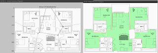Instead of solving within a polygon, the area is treated as a 3 dimensional polyhedral. Previous writings have stayed away from this topic. For the most part because it introduces additional factors that don't generally add enough valuable information to justify the additional computational complexity. Here is one final example of the Physical Security Planner in action. This stadium is comprised of 15 security zones, 35 guard areas and 21 sensor devices (not placed in the pictures below)

A more complex multi-zone example

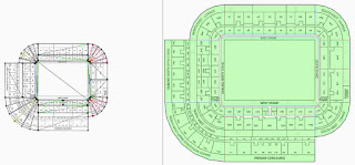Suggested sensor locations for each zone